Graphs and Functions Revision
Graphs and Functions Revision
Graphs and Functions Revision
publish date
Jul 8, 2025
duration
Difficulty
Intermediate
category
UNIT 1/2 Content
UNIT 3/4 Content
what you'll learn
Lesson details
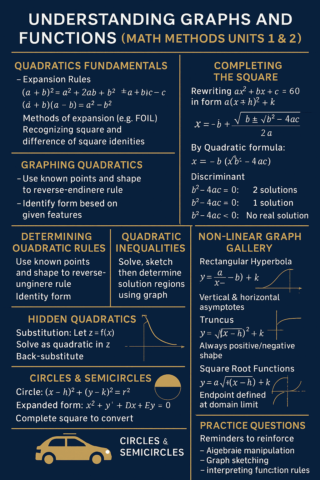
Units 1 & 2 Summary – Mathematical Methods
Unit 1: Quadratics & Coordinate Geometry
1.1 Expanding Quadratics
Use binomial identities to expand expressions to standard form.
1.2 Completing the Square
Rewrite ax^2 + bx + c as a(x + h)^2 + k to identify turning points.
1.3 Solving Quadratics
Solve by factorisation, quadratic formula, and discriminant analysis.
1.4 Graphing Quadratics
Sketch using intercept, turning point, and standard forms.
1.5 Determining Rules
Build equations from known features like intercepts or vertex.
1.6 Quadratic Inequalities
Solve algebraically and verify using graphs.
1.7 Hidden Quadratics
Substitute to reduce complex expressions to standard quadratics.
1.8 Coordinate Geometry
Apply midpoint and distance formulas.
1.9 Gradients and Angles
Use slope and trigonometry to find angles between lines or axes.
1.10 Parallel & Perpendicular Lines
Parallel: same gradient. Perpendicular: gradients multiply to -1.
1.11 Linear Systems
Classify as unique, infinite, or no solution using gradient/y-intercept comparison.
Unit 2: Functions & Calculus in Motion
2.1 Relations and Functions
Functions have one y-value per x; tested with vertical line test.
2.2 Domain and Range
Determine maximal domain and corresponding range (esp. for roots, logs, reciprocals).
2.3 Piecewise Functions
Multiple rules across different domains; must not overlap.
2.4 Inverse Functions
Swap x and y, reflect over y = x, restrict domain if needed.
2.5 Validity of Inverses
Only one-to-one functions have valid inverses.
2.6 Motion Modelling with Calculus
s(t): displacement
v(t) = s’(t): velocity
a(t) = s’’(t): acceleration
2.7 Interpreting Motion Graphs
Slope = rate of change
Area under v(t) = displacement
Area under a(t) = change in velocity
2.8 Solving Motion Problems
Use integration/differentiation with initial conditions.
2.9 Vertical Motion
Model with s(t) = -½gt^2 + v₀t + s₀, solve for max height, time, velocity.
2.10 Technology
Use CAS for differentiation, integration, and graphing motion functions.
About Author